Another simple example of how easy it is to use R in the investment process.
In this case, I’m trying to come up with a way of sorting my target universe to improve stock selection, as opposed to an ad hoc approach to portfolio construction.
The quantmod() library sources four years of fundamental data from Google.
First step is to download and clean the data. (Frankly, the getFinancials() function is of middling value as, for example, much of the income statement items for the Bank sector are NA. In a production environment, a better way to attack the data gathering part of this study would be use Bloomberg and more than four years, and download the data into CSV form for inputting into R.)
Second step: I’m applying a simple Sharpe ratio-type formula of return / standard deviation to the growth rates of the income statement items from each year. The idea is to see which company shows the most consistent growth rate with little variability in Revenue, Net Income, and EPS. With a better data set we could extend this analysis to include gross profit, and perhaps even some balance sheet or cash flow items.
So, we loop through each ticker (I’m using high margin high growth financials for this example) and then generate the Sharpe ratios for each income statement item.
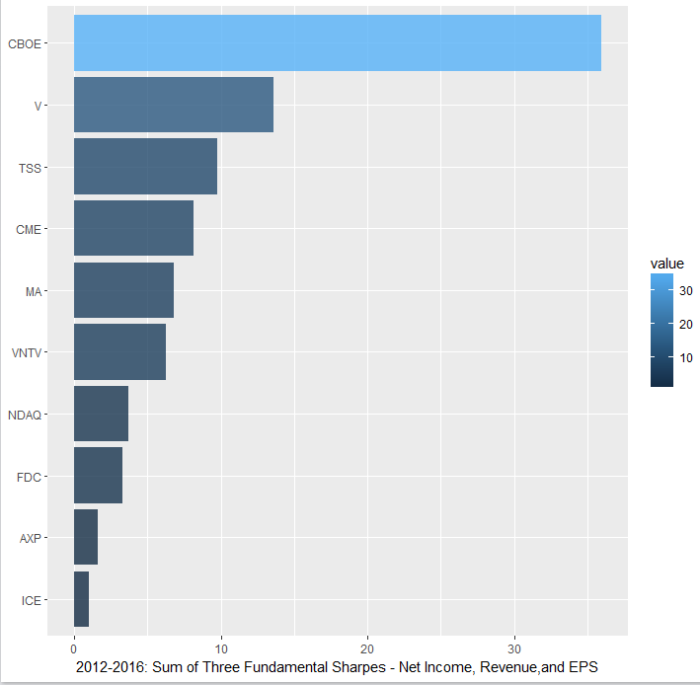
The last step is to somewhat arbitrarily sum the Sharpe ratios, then sort and plot the sums, so we can get a look at the “winner” of this sample data set.
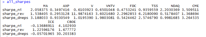
As you can see, ICE and AXP fall to the bottom of the list and CBOE (hmmm worth a closer look at this for reasonableness) and Visa (makes sense) are at the top. The reason, as shown in the second graphic, is ICE has negative Sharpe in net income and EPS, largely due to various acquisitions. Were we to simply sort this by revenues, and/or adjust for acquisitions, the picture might look different.
Bibliography: Financial Analytics with R by Mark Bennett.
library(quantmod)
library(tibble)
d <- 0
mufree <- 0.02
symbols <- c(“MA”,”AXP”,”V”,”VNTV”,”FDC”,”TSS”,”NDAQ”,”CME”,”ICE”,”CBOE”)
stmt <- “A”
basedate=NA
D=length(symbols)
for (d in 1:D) {
symbol <- symbols[d]
getFinancials(symbol,src=”google”)
net_income<-eval(parse(text=paste(symbol,’.f$IS$’,stmt,'[“Net Income”,]’,sep=”)))
base_date <- names(net_income[4])
y4 <- net_income[1]
y3 <- net_income[2]
y2 <- net_income[3]
y1 <- net_income[4]
if (d==1) {
ni_ret <- data.frame(symbol, base_date, y1,y2,y3,y4)
} else {
ni_ret <- rbind(ni_ret,data.frame(symbol, base_date, y1,y2,y3,y4))
}
revenue<-eval(parse(text=paste(symbol,’.f$IS$’,stmt,'[“Revenue”,]’,sep=”)))
base_date <- names(revenue[4])
y4 <- revenue[1]
y3 <- revenue[2]
y2 <- revenue[3]
y1 <- revenue[4]
if (d==1) {
rev_ret <- data.frame(symbol, base_date, y1,y2,y3,y4)
} else {
rev_ret <- rbind(rev_ret,data.frame(symbol, base_date, y1,y2,y3,y4))
}
d_norm_eps<-eval(parse(text=paste(symbol,’.f$IS$’,stmt,'[“Diluted Normalized EPS”,]’,sep=”)))
base_date <- names(d_norm_eps[4])
y4 <- d_norm_eps[1]
y3 <- d_norm_eps[2]
y2 <- d_norm_eps[3]
y1 <- d_norm_eps[4]
if (d==1) {
dneps_ret <- data.frame(symbol, base_date, y1,y2,y3,y4)
} else {
dneps_ret <- rbind(dneps_ret,data.frame(symbol, base_date, y1,y2,y3,y4))
}
}
calc_growth <- function(a,b) {
if(is.na(a) || is.infinite(a) ||
is.na(b) || is.infinite(b) || abs(a) < .001)
return(NA)
if(sign(a) == -1 && sign(b) == -1)
return((-abs(b)/abs(a)))
if(sign(a) == -1 && sign(b) == +1)
return(NA)#((-a+b)/-a)
if(sign(a) == +1 && sign(b) == -1)
return(NA)#(-(a+abs(b))/a)
return(round(abs(b)/abs(a),2)*sign(b))
}
ni_ret_g <- data.frame(ni_ret$symbol,ni_ret$base_date,calc_growth(ni_ret$y2/ni_ret$y1),calc_growth(ni_ret$y3/ni_ret$y2),calc_growth(ni_ret$y4/ni_ret$y3))
colnames(ni_ret_g) <- c(“symbol”,”base_date”,”y2″,”y3″,”y4″)
rev_ret_g <- data.frame(rev_ret$symbol,rev_ret$base_date,calc_growth(rev_ret$y2/rev_ret$y1),calc_growth(rev_ret$y3/rev_ret$y2),calc_growth(rev_ret$y4/rev_ret$y3))
colnames(rev_ret_g) <- c(“symbol”,”base_date”,”y2″,”y3″,”y4″)
dneps_ret_g <- data.frame(dneps_ret$symbol,dneps_ret$base_date,calc_growth(dneps_ret$y2/dneps_ret$y1),calc_growth(dneps_ret$y3/dneps_ret$y2),calc_growth(dneps_ret$y4/dneps_ret$y3))
colnames(dneps_ret_g) <- c(“symbol”,”base_date”,”y2″,”y3″,”y4″)
cols <- c(3,4,5)
sharpe_ni <- apply(ni_ret_g[,cols],1,mean)/apply(ni_ret_g[,cols],1,sd)
sharpe_rev <- apply(rev_ret_g[,cols],1,mean)/apply(rev_ret_g[,cols],1,sd)
sharpe_dneps <- apply(dneps_ret_g[,cols],1,mean)/apply(dneps_ret_g[,cols],1,sd)
all_sharpes <- rbind(sharpe_ni,sharpe_rev,sharpe_dneps)
colnames(all_sharpes) <- ni_ret_g[,1]
z <- colSums(all_sharpes)
tb<-as_tibble(z)
tb$symbol<-ni_ret_g[,1]
tb %>%
filter(value > 1) %>%
mutate(symbol = reorder(symbol, value)) %>%
ggplot(aes(symbol, value, fill = value)) +
geom_bar(alpha = 0.8, stat = “identity”) +
labs(y = “2012-2016: Sum of Three Fundamental Sharpes – Net Income, Revenue,and EPS”,
x = NULL) +
coord_flip()
all_sharpes
The calc_growth function comes from the following excellent book:
https://www.amazon.com/Financial-Analytics-Building-Laboratory-Science/dp/1107150752/ref=sr_1_1?s=instant-video&ie=UTF8&qid=1482169831&sr=8-1&keywords=financial+analytics+with+r